Introduction
The silicon detectors (SSD + SVT) alignment is based on minimization of the residuals between the track projection and the hit positions of all detectors starting from initial survey information. The method utilizes linear approximations to several dependencies between observable quantities and the related alignment parameters. This aproximation requires that any misalignment must be very small. Thus the process is necessarily iterative.Method
- Notations (units are in cm):
- Global: X, Y, Z;
- Local: u (x, drift), w (y), v (z);
- Rotations: α, β, γ, around the local (u,v,w) or global (X,Y,Z), respectively.
- Rigid body model has been applied (ignore possible twist effects for the moment).
- Frozen wafer position on ladder from survey data.
- Misalignment model (D0 model): Taylor's expansion with respect to misalignment parameters
- for 3D shifts:
- (ΔX,ΔY,ΔZ) for global alignment SSD+SVT as whole, or
- (ΔX,ΔY,ΔZ) SVT Shells and SSD Sectors, and
- (Δu,Δw,Δv) for local alignment (Ladders).
- for 3D rotations:
- (Δα,Δβ,Δγ) for global and local.
- for deviations of measured hit position from predicted (from other detectors) primary track position on a measurement plane.
- for 3D shifts:
- A misalignment parameter has been calculated as a slope with straignt line fit of histogram of most probable values for above deviations versus corresponding track coordinates or inclination to detector plane.
Software
Once logged into RCF, the very first step to do
before starting with the alignment procedure is to set the star version
of ROOT to ".DEV2".
starver .DEV2The alignment software contains 2 packages located in $STAR/StRoot/StSvtPool: EventT and SvtMatchedTree

And the corrections obtained with the alignment steps must be put into located in $STAR/StarDb/Geometry:

Eventually, one will not have permission to write on these folders. In this case, the same "directory structure" must be created into the folder where the code is going to be run, i.e., create your StarDb/Geometry/ and put your results there. The code will look for the corrections files first in the current directory and then, if does not find anything, in $STAR/.
Procedures
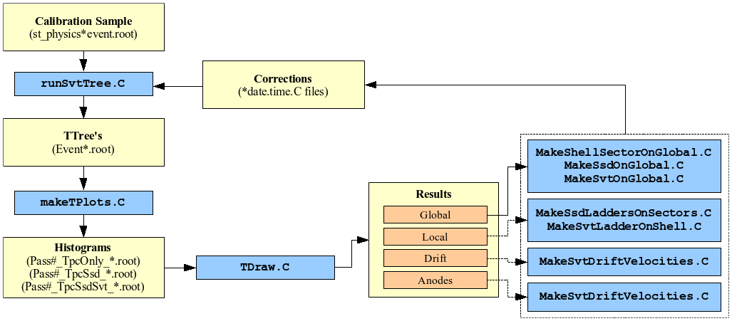
A basic view of the whole procedure is showed in the picture below. Of course, this is a very simplified description and all details regarding each step will be presented afterwards.
This loop must be done as many times as needed to get a "good" result, and also, separately for Global, Local, etc. Once the results have converged, the geometry is frozen and a new sample is generated including the hits of the detector which has just been aligned.
The sequence to be followed for each detector is:
- SSD Alignment: (TPC Only)
- Global;
- Local (ladders);
- SVT Alignment: (TPC+SSD)
- Global;
- Local (ladders);
- Drift Velocities;
- Consistency Check: (TPC+SSD+SVT)
- Global;
- Local (ladders);
- Drift Velocities;
- Getting the Calibration Sample (st_physics_*event.root files):
The calibation sample (*.event.root files) is obtained as result of
standard recostruction procedure with activated SVT and SSD cluster
recostruction and (de)activated tracking recostruction with these
detectors. For CuCu sample (Run V) was used the following chain
options:
- TPC only: "P2005,MakeEvent,ITTF,tofDat,ssddat,spt,-SsdIt,-SvtIt,Corr5,KeepSvtHit,hitfilt,skip1row,SvtMatTree,EvOutOnly"
- TPC+SSD: "P2005,MakeEvent,ITTF,tofDat,ssddat,spt,SsdIt,-SvtIt,Corr5,KeepSvtHit,hitfilt,skip1row,SvtMatTree,EvOutOnly"
- TPC+SSD+SVT: "P2005,MakeEvent,ITTF,tofDat,ssddat,spt,SsdIt,SvtIt,Corr5,KeepSvtHit,hitfilt,skip1row,SvtMatTree,EvOutOnly"
Important !!!! You have to run the above script from directory where you have your StarDb structure
- (Re)Generating the TTree's (Event*.root files): to generate the TTree's, it is needed to run StRoot/StSvtPool/SvtMatchedTree maker with macro StRoot/StSvtPool/SvtMatchedTree/runSvtTree.C.
These TTree's contains primary track predictions for each wafer and all
hits on this wafer. During this step, a set of alignment constants
stored in StarDb/Geometry/svt and StarDb/Geometry/ssd is used. You have to create a TTree for each one of the st_physics*.event.root file, and the easiest way to do this is using the scrip subm.pl to submit jobs. In this script, it is necessary to set the queue name to'star_cas_short' or 'star_cas_prod' (lines 33 and 34, just comment one of them), and then, run the it by typing,
Important !!!! During regeneration of TTree's it is used:- reconstructed track parameters obtained in above reconstruction (which are not changed),
- local SSD coordinates obtained during cluster reconstruction. This allows to change transformation local to global) and
- SVT drift time and anode, which allows to modify local coordinate (drift velocities) and local to global transformation
subm.pl PATH_TO_INPUT_FILES INPUT_FILE_NAMES
Important !!!! You have to run the above script from directory where you have your StarDb structure
The script can handle wild cards (*) and allow you to loop over many files in a given directory. See the example below:

To check whether your jobs were indeed submited, type "bjobs" in the terminal. For more informations about submiting jobs see Using LSF and writing scripts for Batch.
The output files (Event*.root) and logfiles will be saved in the folder from where you submited the jobs. This step usually takes a long time, so, if you like, you can go to take some coffee.
- Histograms (Pass*.root files): in order to create the histograms file, once the jobs submited in the previous step has finished, you have to run the macro makeTPlots.C. To run this macro, just type in a terminal, into the directory where you want the file to be saved, the following command:

You can run just using root (no need for root4star). The macro doesn't take any argument but you tell the code which files to run from the root execution command line. The "| tee" command allows you to send the output file to both the screen and the log file "mylog.log".
The output file appears in the directory where you run from and the file name is as the input with the "/" replaced by "_", example:Pass128/TpcSsdSvt/021/Event*.root ===> Pass128_TpcSsdSvt_021PlotsNFP25rCut0.5cm.root
The next step is do the analysis of the histograms.
Analysis
The analysis of the histograms is done using the macro TDraw.C. This macro allows you to choose the results from Global, Local, Drift and Anodes analysis:- TDraw.C+ returns the Global Alignment results;
- TDraw.C+(5) returns the Local Alignment results (ladders alignment for all barrels, SSD and SVT);
- TDraw.C+(10) returns the Drift Velocities results (SVT hybrids);
- TDraw.C+(20) returns the Anodes results.
- Global: in the directory of the "Pass" which you are working with, create a new directory "Global".
mkdir Global
cd Global
From here, you can run the analysis for Global alignment: TDraw.C+. It takes as input the histogram file created before.root.exe PATH_TO_HISTOGRAM_FILE HISTOGRAM_FILE TDraw.C+
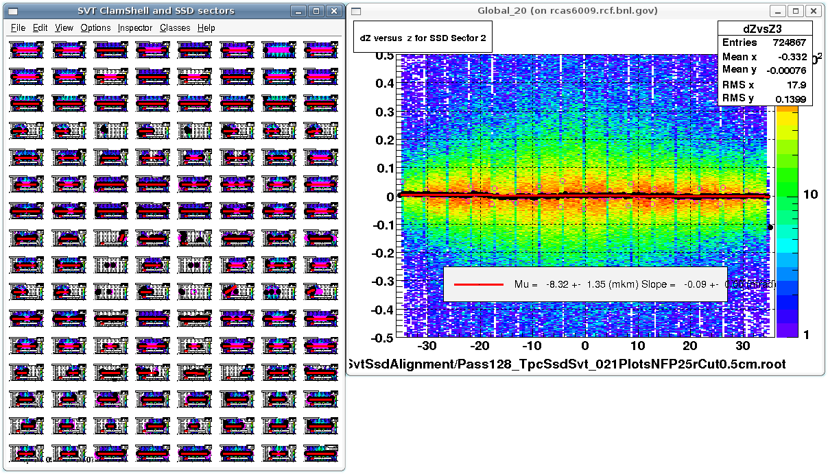
A "Results*" file is produced and also a table of plots showing the fits of all alignment parameters. To see the plots one by one, you can go to "View > Zoomer" and then click with the middle button on the plot you want to see. A common procedure is to save all these plots as web pages, and to do this, go to "File > Save as Web Page", like in the picture below.

Now, you have to check the results. Some derivatives are ill defined and the respective plots will look weird, but do not worry. Grep the average results from the file produced, check whether the values satisfy the following criteria:
- dX, dY, dZ < 10 mkm (microns) or within the standart deviation;
- dα, dβ, dγ < 0.1 mrad or within the standart deviation;

Then, edit the macros,
MakeSvtOnGlobal.C
MakeSsdOnGlobal.C
MakeShellSectorOnGlobal.C
and insert the values in a correction table. The last two rows, Average for All Svt and Average for All Ssd must be put into MakeSvtOnGlobal.C and MakeSsdOnGlobal.C, respectively, and the rows corresponding to SVT Clam Shells and SSD Sector must be put into MakeShellSectorOnGlobal.C. The next picture shows the structure of the table, it is the same for all three macros:

In this structure, it is very important that the entries "date" and "time" agree with the validity period of your data set. You can see the run number of your data set in the name of the files st_physics_<run number>*.event.root and then go to the STAR Online web page to check the informations about the run date. The time stamp is used as a flag for the analysis loop, i.e., the first analysis loop (Global) you set time=000000, then in the second iteraction you put time=000001... in the nth iteraction, time=previous_time+1, and do it up to the final of the whole alignment. It helps you to keep track of what have been done.
After you have edited these macros, you have to run them using root4star.root4star MakeShellSectorOnGlobal.C (example)
Some corrections files will be generated and you will have to copy or move them to $STAR/StarDb/Geometry/svt and $STAR/StarDb/Geometry/ssd (use your StarDb directory if you do not have permission to write in $STAR/).
After that, the corrections obtained will be applied in the next iteraction, so you have to start again from the step (Re)Generating the TTree's. A good advice would be to check the log file produced whether your corrections was found.MakeSvtOnGlobal.C
»
SvtOnGlobal.<date>.<time>.C
MakeSsdOnGlobal.C
» SsdOnGlobal.<date>.<time>.C
MakeShellSectorOnGlobal.C
» ShellOnGlobal.<date>.<time>.C
SsdSectorsOnGlobal.<date>.<time>.C
If you are doing the global alignment for SVT, that means that the SSD geometry has already been frozen, so you must not use the SSD values, just the SVT ones.
- Local: since
you have got good results for the Global Alignment, you can go to Local
Alignment. In the directory of the "Pass" which you are working with,
create a new directory "Local".
mkdir Local
cd Local
Run the analysis for Local Alignment TDraw.C+(5).root.exe PATH_TO_HISTOGRAM_FILE HISTOGRAM_FILE "TDraw.C+(5)"
Results files will be produced for each one of the barrels and also windows with plots of the alignment parameters. The same way as before, save the plots as web pages (View>Zoomer; File>Save as Web page) and check the results. Again, if you have "good" results, you can go to the next step, otherwise, you will have to generate corrections files for the local geometry and run one more time.
The Results* files produced in this case have a pair, Results*.h, which has the correct format required in the macros. You can use them to edit the macros.

Note that the table structure is a little bit different. Althought this table structure does not take into account the date and time flags, you still have to put them in separated variables, and remember that time must follow the sequence from the previous step and date must agree with the validity period of your data set.

The macros which you need to use to generate the corrections files in this case are:root4star MakeSsdLaddersOnSectors.C root4star MakeSvtLadderOnShell.C
You have to run the first one if you are working on the SSD alignment, and the second one if you are working on the SVT alignment.
Copy or move the corrections files for SSD or SVT into the directories $STAR/StarDb/Geometry/ssd or $STAR/StarDb/Geometry/svt, respectively. And after that, go back to the step (Re)Generating the TTree's and do the procedure again in order to try to improve the results.MakeSsdLaddersOnSectors.C
»
SsdLaddersOnSectors.<date>.<time>.C
MakeSvtLadderOnShell.C
» LadderOnShell.<date>.<time>.C
- Drift Velocities (SVT):
after finish the SVT local alignment you also have to check the drift
velocities. In the directory of the "Pass" which you are working with,
create a new directory "Drift".
mkdir Drift
cd Drift
Run the analysis for Drift Velocities TDraw.C+(10).root.exe PATH_TO_HISTOGRAM_FILE HISTOGRAM_FILE "TDraw.C+(10)"
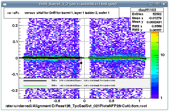
This analysis will produce plots for drift velocities for both hybrids of all wafers of all ladders, and results files for each of the SVT barrels. Each plot (see example below) shows the residual in local x coordinate (u), which is obtained from the drift velocity.

The results files produced in this case (Results*.h) already have the correct table structure, so, to generated the corrections, copy the values into the macro MakeSvtDriftVelocities.C and run using root4star.root4star MakeSvtDriftVelocities.C
The correction file produced is SvtDriftVelocities.<date>.<time>.C and you have to copy or move it to $STAR/StarDb/Calibrations/svt. Then, regenerate the TTree's and do the analysis again to check the results.
- Anodes:
in order to clean up the anodes with bad occupancy, which can produce
wrong results, you have to run the Anodes analysis. So, in the
directory of the "Pass" which you are working with, create a new
directory "Anodes".
mkdir Anodes
cd Anodes
Then, run the analysis for Anodes TDraw.C+(20).root.exe PATH_TO_HISTOGRAM_FILE HISTOGRAM_FILE "TDraw.C+(20)"
The same way as before, a results file is generated (Results*.h) then ... ???
- Comments:
sometimes it is necessary to go back to a previous step to fix some
weird behaviour of some ladders, i.e., you have to go back to ladders
alignment after you have done one iteraction for drift velocities or
anodes.
There is also an effect of magnetic field on position of SSD+SVT with respect to TPC and this effect (at least in the first order) can not be explained by TPC distortions. We see that SSD+SVT moves with switching on/off magnetic field, what means that we have to align the detectors after each change of magnetic field, and this is very important for cases when magnet has tripped.
Bookkeeping
It is very important to keep track of what is done, otherwise one can get lost and the work become confuse and not productive. A very easy way of bookkeeping is to write a file like this README and put it where the final results are been saved, so people can check what have already been done.References
Here, there are some references regarding the alignment method, procedures, and examples:- Results for Cu+Cu data: http://www.star.bnl.gov/~fisyak/star/Alignment
- How-to's: http://www.star.bnl.gov/~fisyak/star/Alignment/HowTo/HowToDoAlignment.html
- Presentation:
http://www.star.bnl.gov/~fisyak/star/alignment/SVT%20calibration%20issues%20and%20remaining%20tasks%20for%20the%20future.ppt
http://www.star.bnl.gov/~fisyak/star/alignment/SVT%20+%20SSD%20calibration%20for%20run%20V.ppt - "Alignment Strategy for the SMT Barrel Detectors", D. Chakraborty, J. D. Hobbs; smtbar01.ps
- "A New Method for the High-Precision Alignment of Track Detectors ", V. Blobel, C. Kleinwort; hep-ex/0208021
- "Estimation of detector alignment parameters using the Kalman filter with annealing", R Fruhwirth et al; 2003 J. Phys. G: Nucl. Part. Phys. 29 561-574
|
Author: Rafael D. Souza
|
Last modified: 04/23/2007 10:26:47 |